What is a system curve?

The system curve describes the relationship between the enclosure's resistance to air and airflow. The physics rule is: resistance is proportional to Q² (Q squared), so the system curve is a parabola starting from the origin and curving upward. Influencing factors: filter density, heatsink fin spacing, intake/exhaust opening area, duct bends, internal obstructions. The same fan in a high-resistance enclosure will operate at a point shifted up-left (lower airflow, higher static pressure); in an open enclosure it shifts down-right (higher airflow, lower pressure).

What is the difference between axial fan and centrifugal fan / blower P-Q curves?

Axial fan P-Q curves are characterized by high airflow but low static pressure — suitable for open or low-resistance enclosures (outdoor cabinets can pair with an intake dust filter), with typical airflow ranges of 50-500 CFM and max static pressure of 2-15 mmH2O. Centrifugal fans / blowers have the opposite characteristic: high static pressure but low airflow — suitable for high-resistance applications such as long ducts, dense fins, and ductwork with multiple bends, with typical airflow ranges of 10-100 CFM and max static pressure of 20-200 mmH2O. Rule: pick axial for low resistance, blower for high resistance.

Where on the P-Q curve should the operating point fall for a valid selection?

The ideal operating point falls in the middle 30-70% region of the P-Q curve, away from both extremes. Too close to the free-delivery point (right end of the curve) means the enclosure is too open and the fan capability is wasted. Too close to the maximum static pressure point (left end) means the enclosure is too restrictive, the fan is near stall, efficiency is low and airflow becomes unstable (axial fans even exhibit a stall region). The middle is the sweet spot for high efficiency, low noise, and high reliability.

Can I buy a fan that only specifies max CFM and has no P-Q curve?

For industrial applications, avoid them. The lack of a P-Q curve usually means either (1) the supplier did not perform wind-tunnel testing (specs are unreliable), or (2) the product is targeted at consumer enthusiasts and not designed with industrial users in mind. Without a P-Q curve, you cannot calculate a real operating point — it's a blind buy. Open-air applications might work, but any enclosure with resistance will trip you up. When sourcing industrial fans, requiring a complete P-Q chart (with at least 5-7 measured points) is the basic industrial standard.

How do I tell if my enclosure's system curve is high-resistance or low-resistance?

Quick three-step check: (1) the ratio of total intake/exhaust opening area to enclosure cross-section — >30% is low resistance, 10-30% is medium, <10% is high; (2) is there a filter, fins, or bent duct in the airflow path — any one of these bumps you to medium resistance or above; (3) is the enclosure packed with components or relatively open — packed (servers, inverters) is high resistance. The most accurate answer comes from a CAE consultancy doing CFD or sending samples through a wind tunnel, but the quick check helps you pick the correct fan type (axial vs blower) up front.

How to Read a Fan P-Q Curve: Static Pressure vs Airflow Engineering Guide

Q: What is the operating point?

The operating point is where the fan P-Q curve intersects the enclosure system curve — it represents the actual airflow + static pressure when the fan is running. The 200 CFM you see in marketing is the free-delivery point (the maximum with zero resistance), but once installed in an enclosure with filters and heatsink fins, the real operating point may drop to just 80 CFM. Always look at the operating point, never the headline CFM.

Q: How does a dirty filter affect the operating point?

A dirty filter raises the entire system curve upward (it takes more pressure to push the same airflow through) — the operating point slides up-left along the fan P-Q curve, and airflow drops. Field experience: when a filter goes from clean to its replacement threshold, pressure drop can increase by 2-5x and airflow can fall by 30-50%. Design recommendation: use the worst-case dirty-filter system curve in your calculations, and reserve a 1.3-1.5x safety margin in your specification.

Q: If I parallel two fans, does airflow double?

No. Parallel operation (two fans installed in the same direction at the same intake) only raises the airflow ceiling, not the pressure ceiling — in a low-resistance system, two fans in parallel deliver about 1.7-1.9x the airflow of a single fan; in a high-resistance system the gain is almost zero. Series operation (two fans head-to-tail) is the opposite — it raises the pressure ceiling but not the airflow ceiling. Series is rarely used in practice (turbulence between fans is complex). When using multiple fans in parallel, you must recompute the system curve and operating point — you cannot extrapolate linearly.

Q: What standards are P-Q curves tested against? AMCA / ISO?

Industrial fan P-Q curves are mainly tested per three standards: AMCA 210 (Air Movement and Control Association, North American industrial standard), ISO 5801 (international industrial fan performance standard), and JIS B 8330 (Japanese industrial standard, common in Asian markets). The three standards differ slightly in chamber geometry, measurement-point layout, and instrumentation, but all share the wind-tunnel + multi-chamber differential pressure measurement principle. When sourcing, a P-Q curve that cites a test standard has high credibility; one that doesn't is usually an internal estimate — confirm with the supplier.

"I bought a 200 CFM fan, why does it only deliver 60 CFM in my cabinet?" This is the most common failure in industrial cooling selection, and 9 times out of 10 the cause is not knowing how to read a P-Q curve. The 200 CFM on the datasheet is the free-delivery point — the maximum airflow with zero resistance. Once installed in an enclosure with filters, fins, and intake/exhaust grilles, the real operating point slides up-left along the P-Q curve and airflow shrinks dramatically. This guide unpacks industrial cooling fan P-Q curves, operating points, system curves, the curve-shape differences between fan types, common mistakes, and 5 typical scenario decisions in one go.

The 60-second answer

Pick a high-airflow type if...

Axial fan, low static pressure, open enclosure

Large intake/exhaust openings, low resistance
Outdoor cabinets can pair with intake dust filter
Mostly empty interior — the job is "moving air"
Typical: IT rooms, open racks, outdoor control cabinets

Pick a high-static-pressure type if...

Centrifugal fan / Blower

Dense fins, long ducts, multiple bends
Enclosure packed with components, high resistance
Need to "push" air through obstructions
Typical: servers, inverters, HVAC ductwork, automotive

Look at the operating point, not max CFM

The core of P-Q curve interpretation

The headline number is a zero-resistance limit
Real performance = "fan curve ∩ system curve"
Valid operating point lies in the middle 30-70%
No P-Q curve = unreliable spec

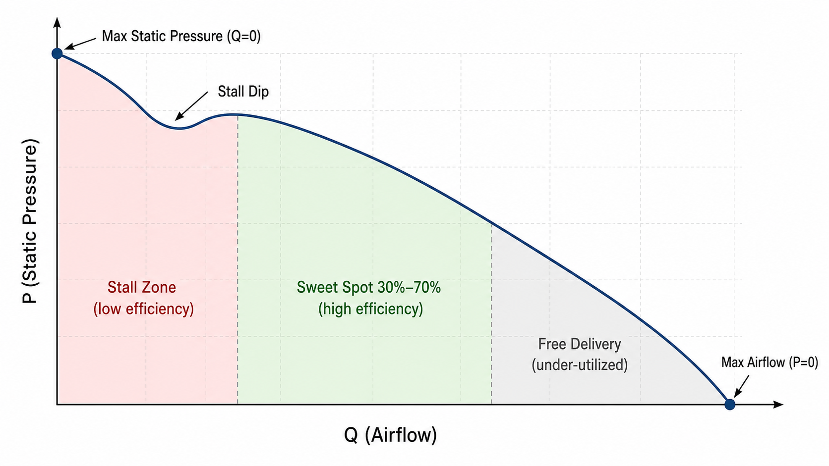
P-Q curve fundamentals

The P-Q curve is the single most important chart on a fan datasheet — more important than max CFM, max RPM, or L10 lifetime — because it tells you the fan's "capability boundary".

Axis definitions

X axis — Q (airflow): in CFM (cubic feet per minute) or m³/min; the volume of air passing through per unit time
Y axis — P (static pressure): in mmH₂O, inH₂O, or Pa; the resistance the fan can overcome

Physical meaning of the two curve endpoints

Position	Physical meaning	Datasheet label
Bottom-right (max Q, P=0)	Free-delivery point — maximum airflow with zero resistance on either side of the fan	"Max Airflow" / "Free-delivery CFM"
Top-left (Q=0, max P)	Shut-off point — maximum static pressure when the outlet is fully blocked	"Max Static Pressure"
Middle region	Normal operating zone — where the fan actually runs	Datasheets usually only mark the endpoints; you need the P-Q chart to see the middle

Many supplier datasheets only give "Max Airflow" and "Max Static Pressure" — that only describes the two endpoints; how the curve behaves between them requires the P-Q chart. A fan without a P-Q chart is like a car spec that gives you only top speed and maximum gradeability, with no torque curve — you have no idea what it can do at any intermediate RPM.

Typical axial fan P-Q curve

Operating point: where two curves intersect

"What the fan can do" is defined by the fan P-Q curve; "what the enclosure demands" is defined by the system curve. The two lines cross at one point — that is the operating point, representing the real airflow + static pressure when the fan is running.

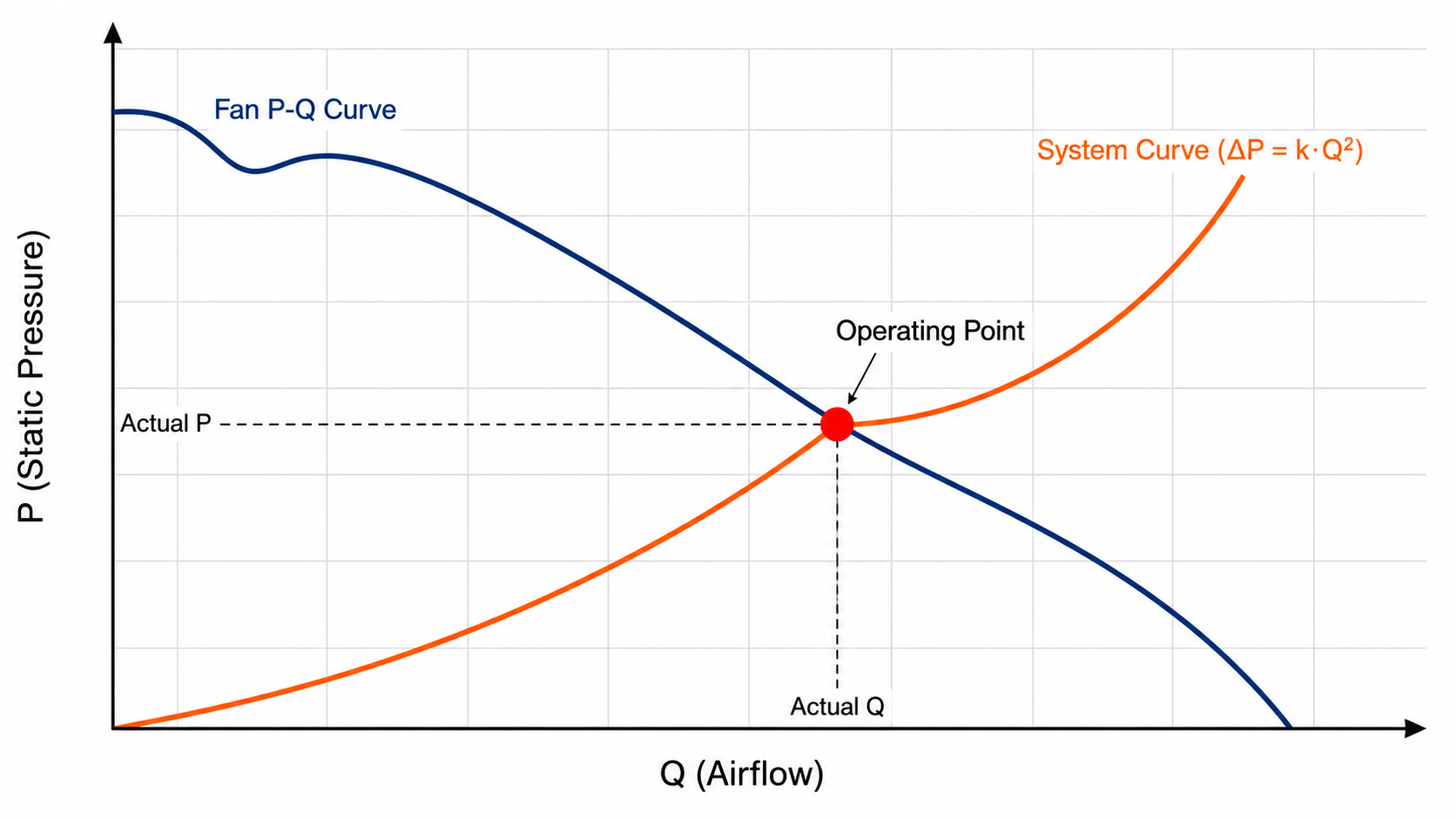
The operating point is the intersection of the fan P-Q curve and the system curve (enclosure resistance), defining the actual airflow and static pressure during real operation. — **Figure 2.** Operating Point = Fan P-Q curve (blue) ∩ System curve (orange, parabolic ΔP = k·Q²). Project the intersection onto the X axis to read Actual Q, project onto the Y axis to read Actual P — the max CFM on the datasheet is not the actual airflow.

The operating point directly determines three things:

Actual airflow — the real number that does the cooling (not the headline CFM)
Actual power consumption — fan power draw at different operating points can vary by 30-50%
Actual noise — the closer the operating point is to the upper-left (high static pressure), the louder the fan typically gets

How the system curve is built

The system curve describes "the relationship between the enclosure's resistance to air and airflow". The physics rule is:

ΔP = k × Q²

In plain English: resistance is proportional to the square of airflow — double the airflow, quadruple the resistance. The system curve is therefore an upward-curving parabola starting at the origin. k is a constant set by enclosure geometry, jointly determined by filter density, fin spacing, intake/exhaust opening area, duct bends, and internal obstructions.

Factors that affect k (resistance magnitude)

Factor	Effect on k	Practical guidance
Total intake/exhaust opening area	Smaller area → k increases sharply	Aim for opening area >30% of enclosure cross-section
Filter density and fouling	Fine filter + dirty → k increases 2-5x	Design with the worst case in mind
Internal obstructions (PCBs, cabling)	The more crowded, the higher k	Reserve sufficient airflow paths
Fin spacing and length	Dense fins + long path → k increases	Heat-exchanger pressure drop of 5-15 mmH₂O is common
Duct bends	Each 90° bend adds 0.5-1.5x the straight-duct pressure drop	Especially important for HVAC ducts

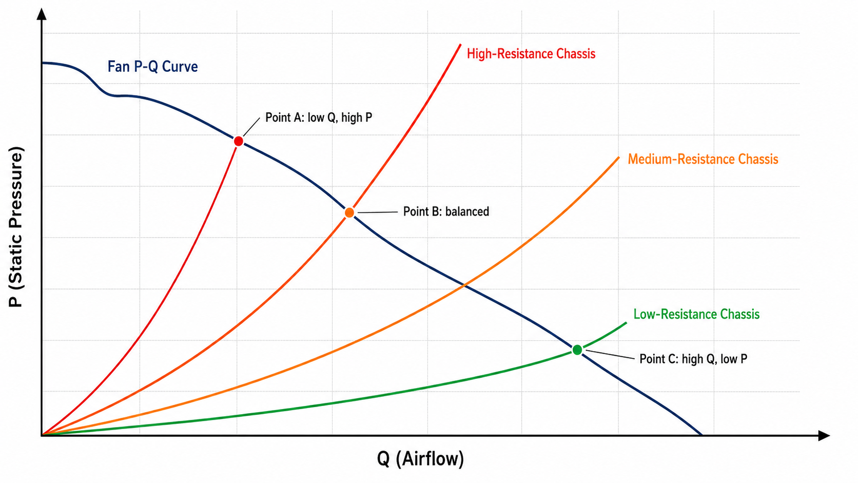
Same fan, different enclosures, very different operating points

The diagram below shows three different operating points for the same axial fan installed in three different enclosures:

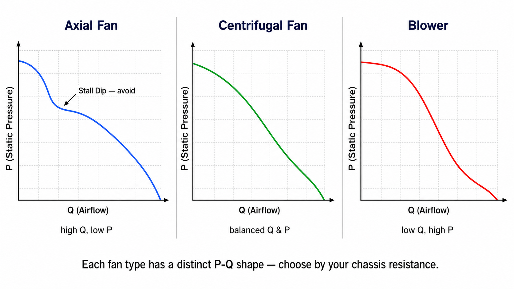
The same axial fan installed in three different-resistance enclosures, with operating points A, B, and C located in different positions on the fan P-Q curve. — **Figure 3.** Same fan, different enclosures, three operating points. **Point A** (red, high-resistance enclosure): low Q, high P, sitting at the edge of the Stall Zone (warning); **Point B** (orange, medium resistance): in the sweet spot, optimal operating position; **Point C** (green, low resistance): high Q, low P, approaching the Free Delivery end — the fan capability is underutilized but if the cooling capacity is sufficient this is still a valid selection.

P-Q shape of three typical fan types

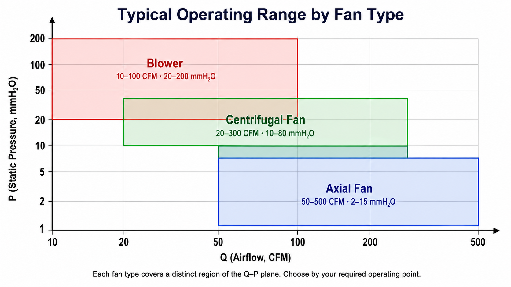
The P-Q curve shapes of different fan types differ greatly, which determines what applications they suit:

Fan type	Typical max Q	Typical max P	Suitable applications
Axial Fan	50 - 500 CFM	2 - 15 mmH₂O	Open / low-resistance cabinets, IT rooms, outdoor cabinets with dust filter, general ventilation
Blower	10 - 100 CFM	20 - 200 mmH₂O	Long ducts, high-resistance cabinets, HVAC ductwork, automotive cooling
Centrifugal Fan	20 - 300 CFM	10 - 80 mmH₂O	Medium-resistance applications, HVAC, mid-size machinery

Side-by-side comparison of axial fan, centrifugal fan, and blower P-Q curve shapes: the axial fan has a stall dip, the centrifugal fan declines smoothly, and the blower shows an S shape. — **Figure 4.** Comparison of P-Q shapes across three fan types. The axial fan has a **Stall Dip** in the middle that must be avoided; the centrifugal fan is a smooth, gentle downward curve; the blower shows an S shape with a flat top and a steep middle drop — the shape differences explain which operating zones each fan type excels in.

Log-log block diagram of the typical operating ranges of three fan types: the axial fan occupies the lower-right (high Q, low P), the blower occupies the upper-left (low Q, high P), and the centrifugal fan sits in the middle and overlaps both. — **Figure 5.** Overlay of typical operating ranges (log-log axes). The **Axial Fan** occupies the lower-right (50-500 CFM × 2-15 mmH₂O); the **Blower** occupies the upper-left (10-100 CFM × 20-200 mmH₂O); the **Centrifugal Fan** sits in the middle and overlaps both (20-300 CFM × 10-80 mmH₂O) — the overlap region means "the same operating point can be reached by multiple fan types", and the choice has to weigh efficiency, noise, and cost together.

Axial fan curve characteristics

An axial fan P-Q curve typically has a stall dip in the middle — when the operating point is pushed near the maximum static pressure, flow separation causes a sudden efficiency drop. Therefore do not run an axial fan near the upper-left of its curve — not only is it noisy, but airflow becomes unstable, efficiency drops, and motor load oscillates.

Blower curve characteristics

The blower P-Q curve is smoother, has no stall problem, and runs stably over a wide range of static pressures. The trade-off is lower airflow than an axial fan of the same size.

Selection decision tree

Estimated operating-point static pressure < 5 mmH₂O → choose an axial fan
Operating point 5-15 mmH₂O → axial fan (38mm thick) or mid-size centrifugal
Operating point 15-50 mmH₂O → centrifugal fan or small blower
Operating point >50 mmH₂O → blower (axial cannot reach this pressure)

Where a valid operating point falls

The ideal operating point lies in the middle 30-70% region of the P-Q curve, away from both ends. Why?

Region	Position	Issue
Right 0-30%	Too close to free delivery	Enclosure too open, fan capability wasted, possible over-spec costing money
Middle 30-70%	Sweet spot	High efficiency, low noise, high reliability ✓
Left 70-100%	Too close to max static pressure	Axial fans may enter the stall region — efficiency drops, noise rises, long-term load oscillation

* The 30-70% rule above is a general guideline for axial fans. Different fan types and different impeller designs have slightly different optimal regions (for example, blowers have a wider effective region). For a specific model, ask the fan supplier to mark the optimal operating zone on the P-Q chart, or validate with a sample test before finalizing the spec.

How to obtain your enclosure's system curve

Three methods, from most accurate to fastest:

Method A: CFD simulation (most accurate, requires expertise)

Use tools such as ANSYS Fluent, SimScale, or Autodesk CFD to build a 3D model of the enclosure, input filter resistance parameters, fin geometry, and intake/exhaust positions, and simulate the pressure drop at different airflow rates. The resulting system curve can be overlaid on the fan P-Q chart to locate the operating point. Pros: accurate; can be completed before the prototype is built. Cons: requires a CFD engineer; one modelling pass takes 2-5 days; software licenses are expensive. CFD work is normally performed by the customer's in-house CAE engineer or by an external CAE consultancy; MAX FLOW does not provide CFD services, but can supply detailed fan performance data (P-Q curves, noise, torque, speed curves) to the customer or consultancy as input data.

Method B: Wind tunnel / fan tester measurement (most direct)

Place the actual enclosure into a wind-tunnel test chamber and measure the pressure required to push different forced airflow rates through it. Equipment: a standard wind tunnel per AMCA 210 / ISO 5801, or an in-house fan tester. Pros: real-world data on a real unit. Cons: needs a physical sample; testing is expensive (an outsourced run is typically NT$ 30,000-100,000).

Method C: Estimation (fastest, large error)

Sum the pressure drops of each resistance source inside the enclosure:

Inlet contraction: estimate from area ratio (10-30% area ratio → roughly 1-3 mmH₂O)
Filter: from the supplier's pressure-drop vs airflow curve (typically 1-5 mmH₂O at rated flow)
Fins / heat exchanger: from supplier spec (5-15 mmH₂O is common)
Duct bends: 0.5-1.5 mmH₂O per 90° bend
Outlet: similar to the inlet

Adding these up gives "total pressure drop at a given reference airflow" — that is one point on the system curve. Then use the ΔP ∝ Q² rule to extrapolate to other airflows.

* Estimation typically carries an error of ±30-50% and is suitable only for preliminary selection. Validate with Method A or B before finalizing the spec, especially for high-density applications (servers, medical equipment, automotive) — a 30% estimation error in those applications translates directly into thermal failures.

5 typical application scenarios

Scenario 1: Open-plan IT room ventilation

Large IT room with partially open rack front and rear doors, where the air-conditioning unit handles the overall temperature and the fans only provide local airflow boost.

→ Choose an axial fan, 120-200mm large size, low-static-pressure type. The system curve is very flat; the operating point falls in the lower-right 60-70% region of the fan P-Q curve (close to free delivery is fine here because there is little resistance to overcome).

Scenario 2: Industrial control cabinet with filter

Outdoor control cabinet with a dust filter at the intake and louvres at the exhaust. The interior is packed with PLCs, relays, and transformers.

→ Choose an axial fan, 120×38mm thick model, high-static-pressure variant. The filter plus internal obstructions make the system curve steep, and the operating point falls in the middle 40-60% of the fan curve. Calculate using a "dirty filter" worst-case scenario and reserve 1.5x margin.

Scenario 3: High-density server rack (1U chassis)

1U server with short front-to-back distance, extremely high PCB density, dense CPU heatsink fins, and very high airflow resistance.

→ Choose 40-60mm high-RPM fans, ultra-high-static-pressure type, multiple fans in parallel. The system curve is very steep and requires small-size, high-RPM fans plus multiple in parallel to overcome the extreme resistance. May be a blower (axial cannot reach this static pressure) or four 60×38mm axial fans in parallel.

Scenario 4: HVAC ductwork system

Commercial-building central air conditioning, with long-distance ducts, multiple bends, and end-of-line filters and diffusers.

→ Choose a centrifugal fan or blower, AC input or EC fan with 0-10V control. Long ducts plus multiple bends plus end filters can accumulate 50-150 mmH₂O of resistance; an axial fan cannot reach this. EC blowers are the standard for HVAC.

Scenario 5: Sealed medical equipment enclosure (CT, MRI control cabinet)

Precision electronics inside medical equipment, requiring low noise, high reliability, and strict thermal margins.

→ Choose 80-120mm axial, hydraulic or ball bearing, low-noise type. The enclosure usually has engineered cooling channels (medium resistance). The system curve is medium-to-steep, and the operating point falls precisely in the 50-60% sweet spot of the fan P-Q curve. Recommend customer-side CAE CFD validation plus a fan-sample acoustic test.

6 most common selection mistakes

Mistake 1: Looking only at max CFM, not the P-Q curve

"A 200 CFM fan" sounds impressive, but that number is at zero resistance. Installed in an enclosure with a filter, you might only get 60 CFM.

Correct approach: ask the supplier for a complete P-Q chart, calculate the enclosure system curve, and find the operating point.

Mistake 2: Calculating with a clean-filter system curve

A dirty filter increases pressure drop by 2-5x, the operating point shifts sharply leftward, and airflow plummets. The equipment overheats a few months into operation.

Correct approach: calculate the system curve using the worst-case "filter due for replacement" condition, and put a filter maintenance schedule in place.

Mistake 3: Assuming two fans in parallel = double the airflow

Parallel operation only approaches 1.7-1.9x in low-resistance systems and barely improves anything in high-resistance systems. Designs assuming 2x and end up undercooled.

Correct approach: when paralleling N fans, overlay the "N × single-fan P-Q curve" (airflow multiplied by N) on the original system curve and find the new operating point.

Mistake 4: Picking an axial fan for a high-static-pressure application

The enclosure pressure drop is 50 mmH₂O, but you bought an axial fan with max P = 8 mmH₂O. It cannot push the air at all.

Correct approach: for high static pressure (>15 mmH₂O), always choose a blower — never force-fit an axial fan.

Mistake 5: Intake/exhaust opening area is too small

The fan inside the enclosure is the right pick, but the intake opening area is only 5% — the bottleneck is the opening, not the fan.

Correct approach: aim for total intake/exhaust opening area ≥30% of the enclosure cross-section; without this, no fan is strong enough.

Mistake 6: Using consumer PC fan specs for industrial applications

PC fan datasheets typically only list max CFM and skip the industrial-grade P-Q chart. Real-world performance in an industrial cabinet falls far short of the headline numbers.

Correct approach: for industrial applications, always pick industrial fans with a complete P-Q curve (AMCA / ISO / JIS test standard).

Frequently asked questions

What is a P-Q curve and how do I read it?

The P-Q curve is the most important chart on a fan datasheet: X axis is airflow Q (CFM), Y axis is static pressure P (mmH₂O). The curve shows the static pressure the fan can produce at any given airflow. The leftmost point is maximum static pressure (when blocked); the rightmost is the free-delivery maximum airflow (zero resistance). The real operating point lies between the two ends and is set by the enclosure resistance.

What is the operating point?

The operating point is where the fan P-Q curve and the enclosure system curve intersect — the real airflow + static pressure when the fan is running. The 200 CFM in marketing is the free-delivery point; once installed in an enclosure with a filter the real operating point may be just 80 CFM. Always look at the operating point, never the headline CFM.

What is the system curve?

The system curve describes "the relationship between the enclosure's resistance to air and airflow". The physics rule is: resistance ∝ Q². The system curve is therefore a parabola starting from the origin and curving upward. Influencing factors: filter density, fin spacing, intake/exhaust opening area, duct bends. The same fan in different enclosures lands on different operating points.

What is the difference between axial fan and centrifugal / blower P-Q curves?

Axial fans are high-airflow, low-static-pressure (max Q 50-500 CFM, max P 2-15 mmH₂O), suited to open or low-resistance enclosures — outdoor cabinets can pair with an intake dust filter. Centrifugal fans / blowers are high-static-pressure, low-airflow (max Q 10-100 CFM, max P 20-200 mmH₂O), suited to long ducts, dense fins, and high-resistance ductwork with multiple bends. Rule: axial for low resistance, blower for high resistance.

Where on the curve should the operating point fall to be valid?

The ideal operating point lies in the middle 30-70% of the curve, away from both ends. Too close to free delivery means the enclosure is too open and the fan capability is wasted; too close to max static pressure means the enclosure is too restrictive, efficiency drops, and an axial fan may stall. The middle is the high-efficiency, low-noise, high-reliability sweet spot.

How does a dirty filter affect the operating point?

A dirty filter raises the system curve as a whole, the operating point slides up-left along the fan P-Q curve, and airflow drops. Field experience: from clean to replacement-due, pressure drop rises 2-5x and airflow can fall 30-50%. Calculate using the worst case during design and reserve a 1.3-1.5x margin.

If I parallel two fans, does airflow double?

No. Parallel operation only raises the airflow ceiling, not the pressure ceiling — in low-resistance systems two fans in parallel give about 1.7-1.9x of one; in high-resistance systems the gain is almost zero. Series operation (head-to-tail) is the opposite — raises pressure but not airflow ceiling. With multiple fans in parallel, recompute the system curve and operating point — never extrapolate linearly.

Can I buy a fan that has only max CFM and no P-Q curve?

For industrial applications, avoid them. The lack of a P-Q curve usually means the supplier did no wind-tunnel testing (specs are unreliable), or the product is positioned at consumers. Without a P-Q curve you cannot calculate a real operating point — open-air applications might be OK, but any enclosure with resistance will trip you up. For industrial fan sourcing, requiring a complete P-Q chart (at least 5-7 measured points) is the basic standard.

How do I tell if my enclosure's system curve is high or low resistance?

Quick three-step check: (1) opening area as a fraction of enclosure cross-section — >30% low resistance, 10-30% medium, <10% high; (2) is there a filter / fin / bent duct in the airflow path — any one bumps you to medium resistance or above; (3) is the interior packed or open — packed (servers, inverters) is high resistance. For accurate results, hire a CAE consultancy to do CFD or send a sample enclosure through a wind tunnel; the quick check helps you pick the right fan type up front.

What standards are P-Q curves tested against? AMCA / ISO?

Three mainstream standards: AMCA 210 (Air Movement and Control Association, North American industrial standard), ISO 5801 (international industrial fan performance test), JIS B 8330 (Japanese industrial standard). The three differ slightly in chamber geometry and measurement-point layout but all share the wind-tunnel + multi-chamber differential pressure measurement principle. When sourcing, a P-Q curve that cites a test standard is highly credible; one without is usually an internal estimate — confirm with the supplier.

Back to Technical Support